
by Lloyd Harris
Every tangible object can be represented with an oval, a rectangle, a triangle, or some combination of the three basic object forms.
When you think about a honey bee colony what shape do you think about? Do you think of a colony as if it were the same shape as the rectangular box that houses the colony?
What shape is your colony in? Everyone has an image in their mind that they use when they define what a honey bee colony is. For most people, the image is a geometric shape of some kind. The more familiar a person is with honey bee colonies the more complex that shape becomes. The beekeeper’s mental image of a colony’s shape is central to understanding what a colony is, how it normally develops, and how colony management practices affect its subsequent development. For some people, the image that they associate with a honey bee colony may be quite simple, or it may be complex, or it may be constructed as a collage of overlapping images.
For the average person with little beekeeping experience, the honey bee colony may be thought of as a triangular or semi-circular, gumdrop-shaped cluster of bees hanging from a tree branch in their backyard; no more, no less.
Those with a little more exposure to honey bees may define their honey bee colony from the physical dimension of the hive bodies surrounding the colony. They may think of the colony as being a stack of rectangular cubes of various heights. For them, the hive and the colony are interchangeable terms for the same thing, but in reality, they are not. The hive is the physical structure surrounding the colony, while the term colony refers to the bees inside the hive.
Understanding a honey bee colony begins with understanding a honey bee’s life cycle and its relationship to colony development.
People who have had a casual look inside a beehive may think of the honey bee colony as being an ellipsoidal blob of bees bisected by a series of wax combs inside one or more rectangular, round, or trapezoidal hive structures.
Usually, people that have actually looked into a beehive and know something about bee biology have a much more complex image they use when they think about a honey bee colony. Their reference image acknowledges that a bee’s life begins as an egg, develops through the larval and the pupal stage and then ends its life as an adult bee. These people think of the colony as being composed of four linear segments placed end to end. The first segment represents the eggs in the colony. The second segment represents the larvae in the colony. The third segment represents the sealed brood (i.e. resting/spinning larvae and pupae). The fourth and final segment represents the adult bees. They think of the colony as being a linear progression of bees progressing from one stage to another as they age. The image that they associate with a honey bee colony may be: a line, a cylindrical tube, or a rectangular tube that has been sub-divided into four sections; the length of which is defined by the duration of each stage (Figure 1).
Figure 1. Linear representation of a honey bee colony showing the developmental progression of honey bees from the egg stage through to the adult bee stage.
Some beekeepers use a slightly different version of the linear model. In addition to dividing the colony into four sections, they further subdivide each of the four segments (developmental stages) based on the duration of each segment (see Figure 2). The egg segment is three days long. The larval segment is about six days long. The resting larvae and pupal stage (sealed brood stage) is 12 days long. The adult bee stage is of somewhat variable length depending on the colony’s health and its environment. The adult segment is divided into up to 320 daily sub-segments. However, many of these daily adult segments will be empty for much of the year. In normal colonies, the bees recruited during April, May, June, July, and the first half of August only occupy, at most, the first ninety-six adult segments. Only bees reared after mid-August and during winter are contained in the adult segments beyond the first 96 segments.
Figure 2. Linear representation of a honey bee colony showing developmental progression of honey bees from the egg stage through to the adult bee stage and the duration of the respective stages.
In the linear system, new bees are added to the colony as eggs. Every day, more bees are added/recruited and the previous day’s eggs and immatures continue to metamorphose until they emerge as adult bees.
The adult bee segments can also be grouped into nurse bees, hive bees, and foragers based on the duties they perform. Worker bees progress through these task related sub-divisions as they age. These sub-division, may not form consecutive pathways. Some bees may perform all the hive related tasks consecutively, one after the other, until they begin foraging. Some bees may perform selected duties for prolonged periods of time before progressing on to another task. Some bees may never perform certain tasks. These temporal related series of duties should be viewed as a series of intertwined pathways of varying lengths. The longer the path is before a bee becomes an active forager, the longer its life will be. After performing a suite of tasks, each bee ultimately exits the colony permanently and dies.
For some beekeepers, this reminds them of a cluster of bees proceeding as a lump from one end of an elastic hose down its length until it exits the other end.
The hose and lump of bees analogy is a good one. This would be what population modellers would refer to as a unidirectional “stock and flow” model. The bees are stocked into one end of the system and flow out the other. However, this analogy is a bit misleading. This hose “leaks” bees as they travel down the length of the hose. Consequently, nothing actually ever flows out of the hose. This analogy can also lead to some misconceptions if one overlooks the fact that another group of bees is added to the colony every day. In reality, a new cluster of bees proceeds down another parallel imaginary hose every day.
Beekeepers familiar with spreadsheets may prefer to view this linear colony representation as a column of cells stacked one above another or end to end. Each spreadsheet cell being a compartment designed to hold however many bees you decide to place into it. The nice thing about spreadsheets is that each compartment can also hold a mathematical formula to aid in determining what each cell contains. The older a bee or a bee cohort becomes; the further it progresses along the “hose”.
The simplest version of the spreadsheet cell analogy generates an image similar to that shown in Figure 3.
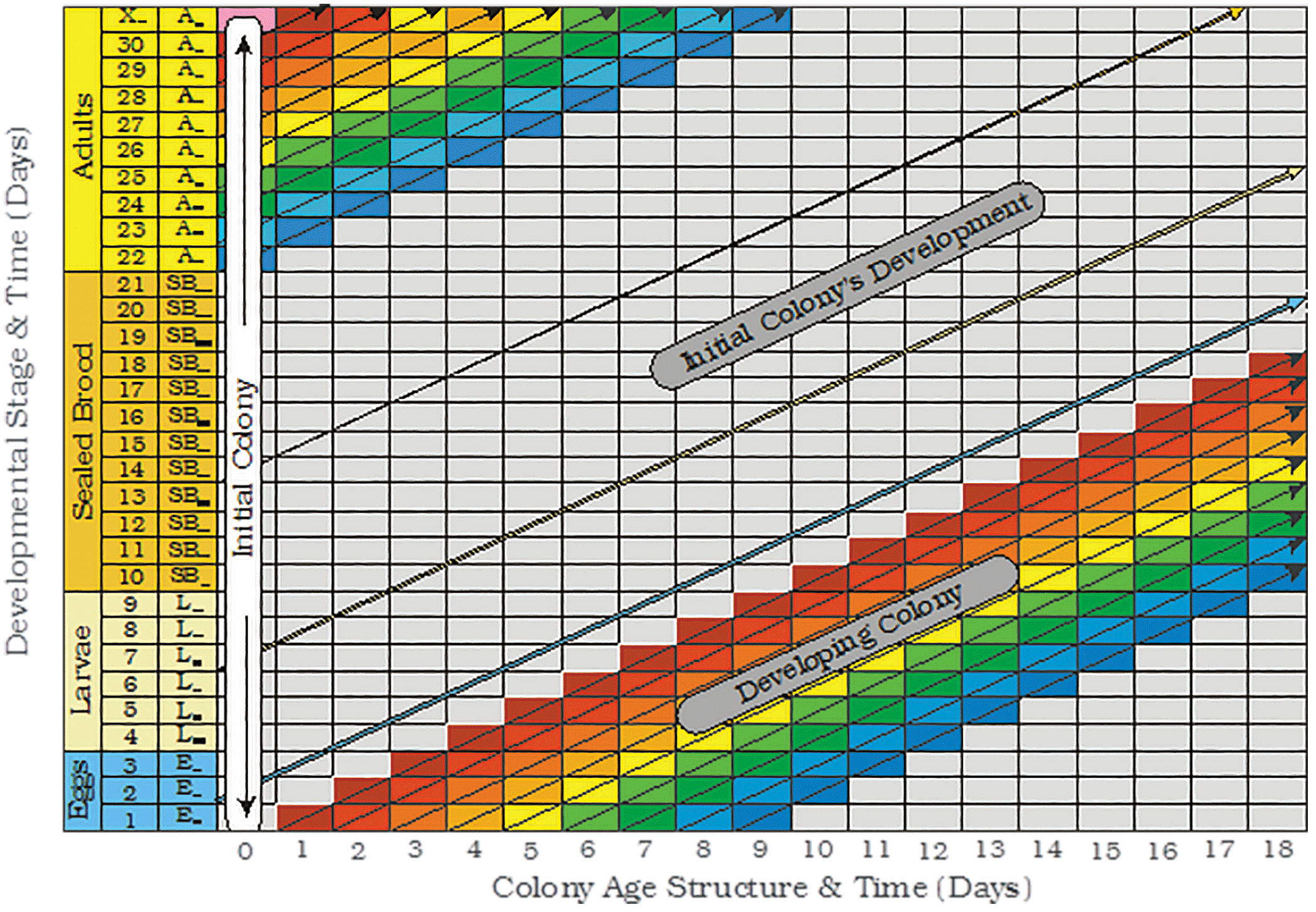
Figure 3. A cellular spreadsheet representation of a developing honey bee colony; where the cells/rows in each column represents eggs, larvae, sealed brood and adults of various ages in the colony on a series.
If a new colony is initiated without brood, a known number of worker bees, and a mated queen; its age structure will be reminiscent of that shown in Figure 3 at Time = 0. When looking at the colony’s initial age structure, it is important to realize that each newly recruited bee cohort is not derived from the age class immediately below them. They are actually derived from the bees added to the colony during some previous day in the past. Each day`s contribution of new bees in the spreadsheet moves diagonally across the spreadsheet rather than just horizontally or vertically.
When this is taken into consideration, the colony can be thought of as being composed of all the bees that were in the colony yesterday plus the bees added to the colony as eggs today. As a consequence, a new image of the colony is formed every day that recognizes that today`s colony is a product of the recent past. The colony is represented by a series of colony images, related in time; each derived from yesterday`s bees plus the bees added to the colony today.
If new bees are continuously added to a colony every day without any interruptions, a cylindrical or rectangular tube image may be an acceptable colony image. However, rather than a single image, the colony might be viewed as a family of images being something analogous to a Russian nesting doll, a musical flue pipe (think pan flute) with its array of parallel stems, or an array of nested cells or overlapping daily sub-populations that can be thought of as being represented as the cross sectional view of a series of stairs arranged one above another (see Figure 3). This image is somewhat incomplete. It is only a partial representation of the colony. It only relates to the development of a hypothetical colony that forms after the first group of eggs are added to the colony at the beginning of their journey down the colony’s daily “pipeline”. To have a complete vision of a colony, the cell contents above the developing colony in Figure 3 also needs to be represented. If they are not accounted for, it will take at least 71 to 95 days in healthy colonies, before the first complete image of the colony would be possible. It takes that long during the Summer for each cohort/sub-population of new bees to die.
“The colony is represented by a series of colony images, related in time; each derived from yesterday’s bees plus the bees added to the colony today.”
To rectify this problem, the size and age structure of the initial colony and its survival must be estimated. At the beginning of the season on some random Day 0 (see figure 3), a colony will start with some variation of the linear model. The initial colony will contain: a queen, a variable number of bees of unknown ages, sealed brood, larvae, and eggs. Typically, a colony begins the season as a package bee initiated colony, a swarm initiated colony, or a broodless wintered colony. It may also begin the season as a wintered colony with brood or as a requeened nucleus colony with brood. Once the initial colony type has been determined, the colony’s initial adult bee population needs to be estimated, and its age structure and survival calculated.
To do this, the spreadsheet must be expanded to the left for at least 84 days or longer if the initial colony has been wintered in a temperate climate. These calculations can by performed by expanding the spreadsheet in Figure 3 into the past or by creating a secondary worksheet, using the same logic used to estimate the developing colony, before transferring the calculations into the main worksheet on Day 0.
The initial colony’s size can be derived reasonably well by estimating the adult bee population by:
- estimating the adult bee population by comparing each frame with photographs containing a known number of bees (Jeffree, 1951; Nelson & Jay, 1972), or
- counting the number of adult bees contained on photographs of the frames,
- weighing the adult bee population and then converting the weight estimate to an adult bee population estimate based in the average weight of a bee (Nolan 1932),
- determining the cumulative percentage frame occupancy and converting these estimates to adult bee estimates based on the number of bees that a frame would be expected to contain if it were completely covered by a dense single-layer of adult bees (ie. Burgett & Burikam, 1985; Imdorf & Gerig, 1999).
“The underlying premise for the DeGrandi-Hoffman et al. (1989) approach to worker bee longevity was based on the fact that a bee’s longevity is affected by the age at which it starts foraging. The younger a bee is when it starts foraging, the shorter its life expectancy will be.”
The colony’s initial age distribution can be approximated, but this requires an understanding of what the colony’s recruitment rate/brood production and survival rates had been.
This basic linear image (figure 4a) is the rudimentary beginning of a very simple population model. It recognises that new individuals are primarily recruited to the colony through the queen’s egg laying activities and that after a period of time these individuals eventually die and no longer form part of the colony. The assumptions of the initial model, although they are not explicitly stated, are that: 1) population recruitment is constant and 2) bees of the same cohort die simultaneously after a specified number of days. Both of these assumptions are not true. However, this rudimentary linear model provides a good starting point from which to build a more complex vision of the colony.
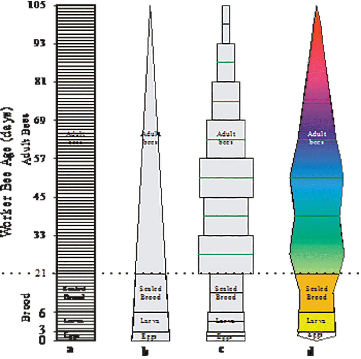
Figure 4a-d. Honey bee colony shape as determined from – a) a colony with a constant daily worker bee recruitment rate, b) a colony with a fixed daily recruitment rate and a relatively constant mortality rate, c) mortality rate, d) item 4c redrawn as a “kite diagram
Perhaps, it would also be more appropriate to think of this simple linear model as being somewhat plastic. A more plastic version of the linear model would be the most preferable image to use when thinking about a honey bee colony. A plastic linear model allows your mind to reshape the colony’s image to accommodate other information that you know that could potentially affect a colony’s shape.
Even if the recruitment rate is constant, the brood portion of the linear image will not have parallel edges because not all the daily recruited bees are likely to survive (see figure 4b). The hose/pipeline leaks. If the adult bees in the colony cannot adequately feed and care for all of the new recruits, they will not be allowed to live. Some may be cannibalized (Fukuda and Sakagami 1968). Other bees may succumb to: American foulbrood, European foulbrood, sacbrood, chalkbrood, various viruses, or Varroa mites. As a consequence, a colony with a constant recruitment rate should not be represented as having parallel sides but rather tapered sides that reflect that not all the bees recruited to the colony will survive to become adults. If a colony has a constant daily recruitment rate, the sides of the first three initial linear segments will not be parallel to each other but rather tapered to reflect the death that occurred in the first 21 days of their life (see figure 4b). Most population models incorporate brood mortality rates observed by Fukuda and Sakagami (1968) because colony specific mortality rates for eggs, larvae and sealed brood are expensive and time consuming to acquire.
Likewise, the shape of the fourth segment containing the adult bees will depend on when these adult bees die. Adult bees emerging in a healthy colony between 1 April and mid-August on the Northern Great Plains of North America, should have an average adult life expectancy of between 33.3 to 36.5 days or slightly higher. Less than 0.06 percent of the spring and summer reared adult bees survive until they are between 84 and 96 days of age (Harris & Harris, unpublished).
Nolan (1932) used a hypothetical worker bee longevity to estimate a colony’s adult bee population. It was based on a division of labour proposed by Rösch (1925), where: the average adult bee spend two days cleaning cells, eight days nursing young bees, nine days performing other hive duties, and the last 16 days of their adult lives as foragers before they die. In essence, in his model, the adult bee population was assumed to contain exactly 35 daily adult bee segments. When a bee became 36 days old, it died. Bodenheimer (1937) used a similar assumption, except the adult portion of the colony contained 42 daily adult bee segments. The total life expectancy of a worker bee from the time it was deposited as an egg until it died was estimated to be exactly 63 days.
This allowed Bodenheimer (1937) to construct the first graphical representation showing the theoretical age distribution for a honey bee colony. Although the colony shapes proposed by Bodenheimer are interesting, they are not very enlightening because the assumptions used to create them were not realistic.
“In a healthy colony, maximum life expectancy for bees emerging as adults during the Summer is at least 84 days but always less than 96 days.”
DeGrandi-Hoffman et al. (1989) determined the duration of the adult bee population by assuming that the bees functioned as hive bees until they were 21 days old (Free, 1965) and that they were then removed from the adult population after foraging for a fixed number of bee foraging days determined by the model’s user. Bee-foraging days were defined as any day when the average temperature exceeded 12oC (Lundie, 1925), wind velocity was less than 34 km/h (Rashad, 1957) and rainfall was less than 0.5cm. The underlying premise for the DeGrandi-Hoffman et al. (1989) approach to worker bee longevity was based on the fact that a bee’s longevity is affected by the age at which it starts foraging. The younger a bee is when it starts foraging, the shorter its life expectancy will be (Rueppell et al. 2007).
Any theoretical variation on the basic scheme is possible. You know that bees do not simply die in unison once they reach a certain age. Consequently, having the adult bees “leap” from the top of the colony’s age structure and die in synchrony once they reach some arbitrary, magical age should be rejected. Once, this assumption is rejected as being unrealistic, it needs to be replaced with either a different assumption of when and how bees die or with real data.
Even if you know nothing about how long an average bee lives before it dies, you can still reshape your image of what a honey bee colony looks like. The easiest assumption to make is that worker bees die at a constant rate after they reach some arbitrary age. The rate you pick will determine how many days you let your oldest bee live (see figure 4b).
In a healthy colony, maximum life expectancy for bees emerging as adults during the Summer is at least 84 days but always less than 96 days (Harris & Harris, unpublished). However, adult bees infected with Nosema diseases (Hassanien, 1952) or parasitized by Varroa mite (De Jong and De Jong, 1983) will live much shorter lives.
Ideally, you would use locally derived worker bee longevity estimates from the survival of newly emerged bees that had been marked with distinctive coloured makings (Harris, 1979). However, honey bee longevity estimates from England (Free and Spencer Booth, 1959) the United States of America (El-Deeb, 1952), Japan (Sekiguchi & Sakagami, 1966; Sakagami & Fukuda, 1968) or Canada (Harris & Harris, unpublished) may be used if deemed appropriate. Regardless of what you select as an acceptable honey bee longevity estimate, the result will be that you will have reshaped what your colony looks like. Instead of having the adult bees being represented as a rectangular image (see figure 4a), it will now be triangular (Figure 4b). If you draw your mental image of your colony in three dimensions, it could also be imagined as being conical or polyhedral.
Now, consider a colony where new bees are not added to the population at a constant rate. If your colony’s recruitment rate increases or decreases, this will affect the number of bees in each subsequently derived sub-population of bees as they progress through the colony’s age structure. The more bees a sub-population contains, the wider its representation will be.
The colony’s shape is defined by the numbers of eggs laid in a colony every day and the durations of the bees’ lives. These two variables also determine the number of bees in the colony on any given day. The colony’s population increases when more bees are added to the colony than exit, drift into an adjacent colony, or leave the colony as part of a departing swarm. When more bees die than are recruited, the colony becomes smaller. If you are focused on the adult bee portion of a colony’s population, there will always be a 21 day lag before recruitment changes are reflected in the colony’s adult bee population.
The above logic forms the basic building blocks for most colony population models. The magnitude of the daily recruitment may be defined as a function of the colony’s daily adult bee population, the queen’s reproductive potential, available space, ambient temperatures, or resource availability. A colony cannot produce new worker bee recruits without having a mated queen. The queen cannot produce new worker bee recruits unless the colony has enough nurse bees to feed the queen. The developing brood cannot survive if there are not enough nurse bees to feed and care for them. The nurse bees cannot sustain their activities unless there are foragers collecting the resources that the nurse bees need to rear the brood. Perhaps the most important factors regulating the addition of new recruits to the colony are all external to the colony. Favourable ambient temperature, photoperiod, rainfall, and the presence of pollen and nectar secreting plants in close proximity to a colony are essential factors that determine a colony’s actual recruitment. In managed honey bee colonies, the often overlooked variable affecting colony development is the beekeeper’s effect on bee recruitment and death.
The basic model has been used either as a theoretical predictive tool, or as an applied experimental tool. The two methods manipulate the data differently.
The theoretical models generate colony population estimates by regulating colony development as a function of changes in the cohorts of new bees recruited every day to the colony and applying a mortality rate to the daily recruitment rate. The rate of recruitment is usually a function of: the queen’s egg laying ability, the number of bees in the colony, ambient temperature, growing degree days, photoperiod, nutrient availability, etc.
The applied experimental approach uses a slightly different approach. Instead of determining how many daily recruits are added to, or subtracted from, the colony using theoretical considerations, the applied approach adds its recruits to the colony every twelfth day based on the amount of sealed brood a colony actually produces in response to a host of fluctuating environmental variables. This is the colony’s actual cumulative effective recruitment rate assessed at regular repetitive 12-day intervals. Daily recruitment rates can also be derived from the 12-day interval assessments if necessary.
The applied experimental approach uses sealed brood estimates rather than measuring eggs or larvae because sealed brood is easier to measure. It is also more cost effective and ensures that the new bee recruits are not overlooked nor are they counted twice (Fukuda, 1971). Sealed brood estimates are then converted to bee estimates based on the cells per unit area measurement.
The number of eggs and larvae in the colony are then determined by multiplying the effective daily recruitment rate by the duration of the respective stages and correcting for mortality that may have occurred during each stage. The egg and larval estimates are offset by -12 days because they represent the eggs and larval rates that existed before the sealed brood was measured. The adult bee cohort emerging from the sealed brood stage is also corrected for stage related mortality. The survival of each emerging adult bee cohort/sub-population is determined from the average survival of a series of differently colour-marked newly-emerged bees. The experimental method generates population estimates and colony age distributions (Harris, 2008a, 2008b, 2009, 2010) at twelve day intervals, although daily estimates are also possible.
This method estimates the average number of bees in the egg stage, the larval stage, the sealed brood stage and the adult stage. The number of adult bees in a colony is determined from a series of 12 day age-classes/sub-populations of adult bees staggered by 12 day intervals as they progress along the hypothetical staircase in Figure 3.
The procedure allows the user to calculate eggs, larvae, sealed brood, and adult bee estimates for a colony and its demographics. Colony demography is most useful when determining the potential number of nurse bees or foragers in a colony or when determining when the bees are reared that form the Winter colony (Mattila et al., 2001; Harris, 1980, 2008a, 2008b).
A colony’s demography is best represented with a “kite diagram”. The kite-diagram is formed by first stacking and centering the respective bee estimates above each other; starting with the eggs in the colony and ending with the oldest bees in the colony (figure 4c). The width of each rectangular box represents the number of bees it contains. If you draw a line at the mid-point of these rectangular boxes and connect the ends of the lines, the colony will be represented as “kite diagram” (see figure 4d). The kite diagram can be transformed/splined into a three dimensional image of the colony if you have access to the appropriate drafting software (3D Studio Max®, Autocad®, SolidWorks®, etc.).
Although this applied method is intended for data processing, the basic framework can also be modified to generate limited insight into colony development by altering sealed brood data or the associated survival data.
For example, suppose you are interested in knowing how many bees an average colony needs to produce to maintain its population at its current state (see Harris, 2010). The answer will depend on what the colony’s worker bee longevity is. If the average worker bee longevity is 35.52 days (Harris & Harris unpublished), the colony would need to produce 28.6 new bees per day per 1000 bees to maintain this colony at this equilibrium point. If its average worker bee longevity was 26 days (Rueppell, et al. 2007), the colony would have to produce 36 new adult bees per day. Obviously, anything that reduces worker bee longevity will also reduce colony size unless the colony is capable of compensating for the change by rearing more bees.
Similarly, suppose you want to understand the impact of brood production in September, October, or during winter on a colony’s Spring population. Changing the experimental data or inserting theoretical brood production values will allow you to predict how populous a colony would be in spring. The applied methodology can also be used to verify the accuracy of the various theoretical models.
Good population models always provide the user with a list of the assumptions used by the model. A model’s ability to mimic reality depends on its ability to adequately describe how all the variables affect colony development. Some variables have a direct effect on colony development. Other variables only affect colony development indirectly or in concert with other variables. Most variables only affect colony development between prescribed ranges.
If a model’s assumptions are unrealistic or wrong, then it is almost certain that it will be unable to generate realistic predictions. The vernacular phrase used to summarize this situation has been, garbage in garbage out”. Model complexity depends on: the number of variables considered, the relationships defined between them, and their effects on colony recruitment and bee mortality. Schmickl & Crailsheim’s (2007) HoPoMo Model is a sophisticated version of the basic spreadsheet model.
The method you use to form a mental image of a colony is entirely up to you. If you understand differential calculus, one of the theoretical models may be of interest to you (Martin, 1998, 2001; Ghamdi & Hoopingarner, 2004; Ratti et al., 2012; Khoury et al., 2011, 2013; Becher et al., 2014). If you like using spreadsheets, the applied methods may be of interest. Both methods assist you with determining what shape your colony is in and whether you should change your management practices to get the shape that works best for you and your bees.
References
BECHER, M. A.; GRIMM, V.; THORBEK, P.; HORN, J.; KENNEDY, P. J. and OSBORNE, J. L. (2014) BEEHAVE: a systems model of honeybee colony dynamics and foraging to explore multifactorial causes of colony failure. Journal of Applied Ecology 51: 470–482.
BODENHEIMER, F. S. (1937) Studies in animal populations II. Seasonal population trends of the honey-bee. Quarterly Review Biology 12(4) 406-425.
BURGETT, M. and BURIKAM, I. (1985) Number of Adult Honey Bees (Hymenoptera:Apidae) Occupying a Comb: A Standard for Estimating Colony Populations. Journal of Economic Entomology 78: 1154-1156.
DE YONG, D. and DE YONG, P. H. (1983) Longevity of Africanized honey bees (Hymenoptera: Apidae) infested by Varroa jacobsoni (Parasitiformes: Varroidae). Journal of Economic Entomology 76: 766-768.
EL-DEEB, A. A. (1952) Longevity of some races of the honeybee (Apis mellifera L) Ph.D. Thesis, Illinois State University, Urbana, Illinois.
FREE, J. B. and SPENCER-BOOTH, Y. (1959) The longevity of worker bees (APISMELLIFERA). Proceedings of the Royal Entomological Society of London. (A) 34: 141-149.
FUKUDA, H. and SAKAGAMI, S. F. (1968) Worker brood survival in honey bees. Researches on Population Ecology 10: 31-39. http://hdl.handle.net/2115/27519
FUKUDA, H. (1971) Improvement of Bodenheimer’s Method for Estimating Individual Number in Honeybee Colonies. Journal of the Faculty of Science Hokkaido University Series VI. Zoology, 18(1): 128-143.
GHAMDI, A. A. and HOOPINGARNER, R. (2004); Modeling of Honey Bee and Varroa Mite Population Dynamics. Saudi Journal of Biological Sciences. 11:1.
HARRIS, J. L. (1979) A Rapid Method for Colour-Marking Single Honeybees with Fluorescent Paint. Journal of Apiculture Research 18: 201-203.
HARRIS, J. L. (1980) A population model and its application to the study of honey bee colonies. University of Manitoba, MSc. thesis, 104 pgs.
HARRIS, J. L. (2008a) Development of honey bee colonies initiated from package bees on the northern Great Plains of North America. Journal of Apicultural Research and Bee World 47(2): 141-150.
HARRIS, J. L. (2008b) Effect of Requeening on Fall Populations of Honey Bees on the northern Great Plains of North America. . Journal of Apicultural Research and Bee World 47(4): 271-280.
HARRIS, J. L. (2009) Development of honey bee colonies on the Northern Great Plains of North America during confinement to winter quarters. Journal of Apicultural Research and Bee World 48(2): 85-90.
HARRIS, J. L. (2010) The effect of requeening in late July on honey bee colony development on the Northern Great Plains of North America after removal from an indoor winter storage facility. Journal of Apicultural Research and Bee World 49(2): 159 – 169.
HARRIS, J. L. and HARRIS A. W. (unpublished) Longevity of Worker Honey Bees on the Northern Great Plains of North America.
HASSANEIN, M. H. (1952) The influence of infection with Nosema Apis on the activities and longevity of the worker honeybee. Annuals of Applied Biology 40: 418-423.
IMDORF, A. and GERIG, L. (1999) Course in Determination of Colony Strength. www.agroscope.admin.ch/imkerei/00000/00294/…/index.html.
JEFFREE, E. P. (1951) A photographic presentation of estimated numbers of honeybees (Apis mellifera) on Combs in 14 x 8 inch frames. Bee World. 32: 89–91.
KHOURY, D. S.; BARRON, A. B. and MYERSCOUGH, M. R. (2013) Modelling food and population dynamics in honey bee colonies. PLoS ONE, 8, e59084.
KHOURY, D. S.; MYERSCOUGH, M. R.; and BARRON, A. B. (2011) A quantitative model of honey bee colony population dynamics. PLoS ONE, 6, e18491.
LUNDIE, A. E. (1925) The flight activities of the hoe bee. United States Department of Agriculture Bulletin 1328, 37 pp.
MATTILA, H. R.; HARRIS, J. L.; and OTIS, G. W. (2001) Timing of production of winter bees (Apis mellifera) colonies. Insectes Sociaux 48, 88-93.
MARTIN, S. J. (1998) A population dynamic model of the mite Varroa jacobsoni. Ecological modelling 109:267-281, 1998.
MARTIN, S. J. (2001) The role of Varroa and viral pathogens in the collapse of honeybee colonies: a modeling approach. Journal of Applied Ecology 38:1082-1093.
NELSON, D. L. and Jay, S. C. (1972) Estimating number of adult bees on Langstroth frames. The Manitoba Entomologist 6:5-8.
NOLAN, W. J. (1925) The Brood-rearing cycle of the Honey bee. Department Bulletin 1349, United States Department of Agriculture – 56 pages.
NOLAN, W. J. (1932) The Development of Package-Bee Colonies. Technical Bulletin 309, United States Department of Agriculture.
RASHAD, S. E. (1957) Some factors effecting pollen collection by honey bees and pollen as a limiting factor in brood rearing and honey production Ph.D thesis, Kansas State College, Manhattan KS, 88 pp.
RATTIL, V.; KEVAN P. G. and EBERL H. J. (2013) A mathematical model for population dynamics in honeybee colonies infested with Varroa destructor and the Acute Bee Paralysis Virus. Canadian Applied Mathematics Quarterly 21: 63 – 93.
ROSCH, G. A. (1925) Untersuchugen uber die Arbeitsteilung im Bienenstaat. 1-Die Tatigkeiten in normalen Bienenstaate und ihre Beziehungen zum Alter der Arbeitsbienen. Zeitschrift für vergleichende Physiologie 571-631.
RUEPPELL, O.; Bachelier, C.; Fondrk, M. K. and Page, R. E. Jr. (2007) Regulation of life history determines lifespan of worker honey bees (Apis mellifera L.) Experimental Gerontology 1020 – 1032 doi: 10.1016/j.exger.2007.06.002.
SAKAGAMI, S. F. and FUKUDA, H. (1968) Life tables for worker honeybees. Researches in Population Ecology. 10:127-139.
SEKIGUCHI, K. and SAKAGAMI, S. F. (1966) Structure of foraging population and related problems in the honeybee, with considerations on the division of labour in bee colonies. Report No. 69. Hokkaido National Agricultural Experimental Station.
SCHMICKL, T. and CRAILSHEIM, K. (2007) HoPoMo: A model of honeybee intracolonial population dynamics and resource management (2007) Ecological Modelling 204: 219-245.
Acknowledgements: The foregoing material is an explanation and discussion of the honey bee population estimation methods used in the analysis of a Honey Bee Sentinel Hive Study funded be Bayer CropScience at 6 apiaries in western Canada during the summer of 2014 and the spring of 2015.
A special thanks to Julia Common for her assistance in the development of the visual concepts presented and to Maryam Sultan and Sandra Shiels for their editorial comments.